Double Segmentation#
This page demonstrates how to use tab-right’s double segmentation functionality to analyze model performance across combinations of two features.
What is Double Segmentation?#
Double segmentation allows you to analyze how your model performs across different combinations of two features. This is useful for:
Identifying feature interactions affecting model performance
Finding specific feature value combinations where your model underperforms
Understanding complex patterns single-feature analysis might miss
Tab-right’s Double Segmentation Tools#
Tab-right provides these tools for double segmentation analysis:
DoubleSegmentationImp- Main class for performing double segmentationDoubleSegmPlotting- Visualization with support for both interactive Plotly and static Matplotlib backends
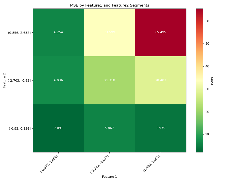
Basic Usage with Continuous Features#
Here’s a simple example of double segmentation with tab-right using continuous features:
import numpy as np
import pandas as pd
import matplotlib.pyplot as plt
from sklearn.metrics import mean_squared_error
from tab_right.segmentations import DoubleSegmentationImp
from tab_right.plotting import DoubleSegmPlotting

# Create sample data
np.random.seed(42)
n_samples = 500

# Generate features and target
feature1 = np.random.normal(0, 1, n_samples)
feature2 = np.random.normal(0, 1, n_samples)

# Target with interaction effect
target = 2 + feature1 + feature2 + 2 * (feature1 * feature2) + np.random.normal(0, 1, n_samples)

# Prediction missing the interaction term
prediction = 2 + feature1 + feature2 + np.random.normal(0, 1, n_samples)

# Create DataFrame
df = pd.DataFrame({
    'feature1': feature1,
    'feature2': feature2,
    'target': target,
    'prediction': prediction
})

# Perform double segmentation
double_seg = DoubleSegmentationImp(
    df=df,
    label_col='target',
    prediction_col='prediction'
)

# Apply segmentation with 3 bins for each feature
result_df = double_seg(
    feature1_col='feature1',
    feature2_col='feature2',
    score_metric=mean_squared_error,
    bins_1=3,
    bins_2=3
)

# Visualize results with a heatmap
plotter = DoubleSegmPlotting(df=result_df, backend="matplotlib")
fig = plotter.plot_heatmap()
plt.title("MSE by Feature1 and Feature2 Segments")
(Source code, png, hires.png, pdf)

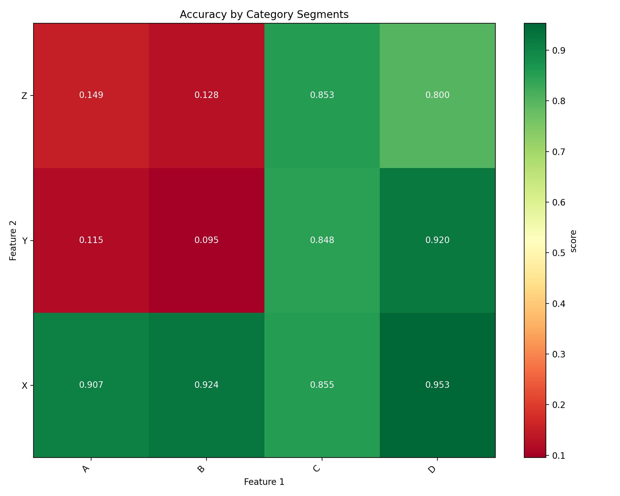
Working with Categorical Features#
Double segmentation works with categorical features without needing to specify bins:
import numpy as np
import pandas as pd
import matplotlib.pyplot as plt
from sklearn.metrics import accuracy_score
from tab_right.segmentations import DoubleSegmentationImp
from tab_right.plotting import DoubleSegmPlotting

# Create sample categorical data
np.random.seed(42)
n = 800

# Generate categorical features with non-uniform distributions
category1 = np.random.choice(
    ['A', 'B', 'C', 'D'],
    n,
    p=[0.4, 0.3, 0.2, 0.1]  # Different probabilities for each category
)
category2 = np.random.choice(
    ['X', 'Y', 'Z'],
    n,
    p=[0.5, 0.3, 0.2]
)

# Generate target with different patterns for combinations
target = np.zeros(n, dtype=int)

# Add different effects for different combinations
target[(category1 == 'A') & (category2 == 'X')] = 1
target[(category1 == 'B') & (category2 == 'Y')] = 1
target[(category1 == 'C') & (category2 == 'Z')] = 1
# Special case with stronger effect
target[(category1 == 'D') & (category2 == 'Z')] = np.random.binomial(1, 0.8, np.sum((category1 == 'D') & (category2 == 'Z')))

# Add some noise
noise_mask = np.random.choice([True, False], n, p=[0.1, 0.9])
target[noise_mask] = 1 - target[noise_mask]

# Simple prediction without capturing all patterns
prediction = np.zeros(n, dtype=int)
prediction[category1 == 'A'] = 1
prediction[category2 == 'Z'] = 1

# Create DataFrame
cat_df = pd.DataFrame({
    'category1': category1,
    'category2': category2,
    'target': target,
    'prediction': prediction
})

# Perform double segmentation
cat_seg = DoubleSegmentationImp(
    df=cat_df,
    label_col='target',
    prediction_col='prediction'
)

# Apply segmentation (no bins needed for categorical features)
cat_results = cat_seg(
    feature1_col='category1',
    feature2_col='category2',
    score_metric=accuracy_score
)

# Plot with higher is better for accuracy
cat_plot = DoubleSegmPlotting(
    df=cat_results,
    lower_is_better=False,
    backend="matplotlib"
)
fig = cat_plot.plot_heatmap()
plt.title("Accuracy by Category Segments")
(Source code, png, hires.png, pdf)

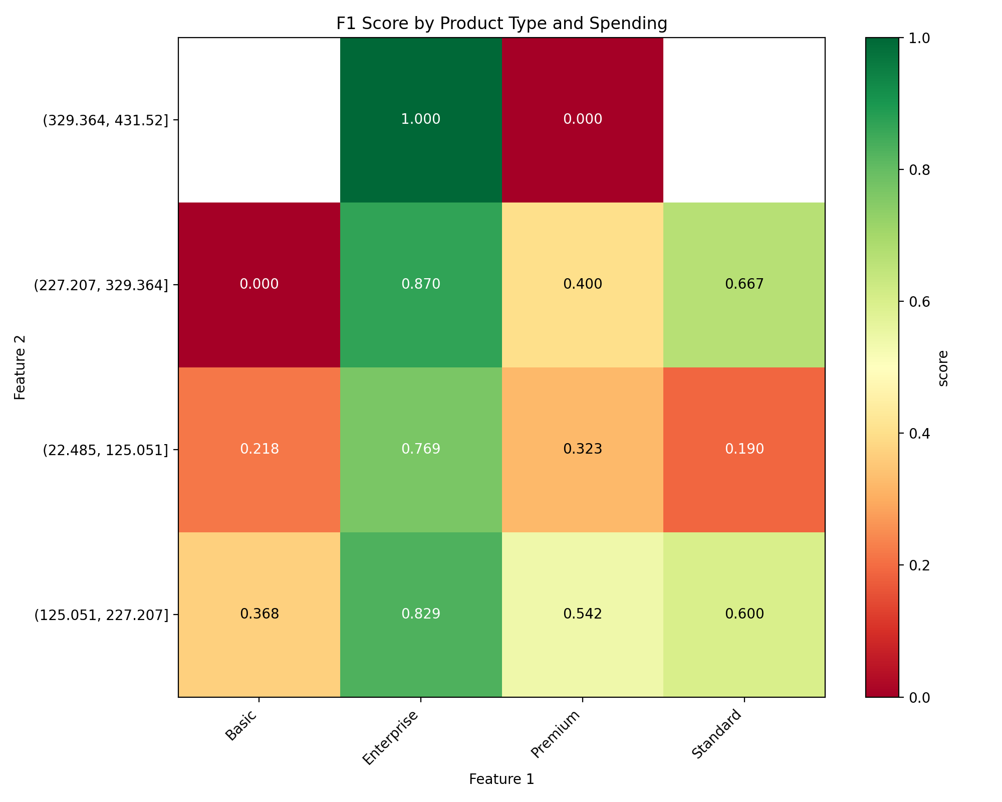
Mixed Categorical and Continuous Features#
Double segmentation can analyze combinations of categorical and continuous features:
import numpy as np
import pandas as pd
import matplotlib.pyplot as plt
from sklearn.metrics import f1_score
from tab_right.segmentations import DoubleSegmentationImp
from tab_right.plotting import DoubleSegmPlotting

# Create sample data with mixed feature types
np.random.seed(42)
n_samples = 500

# Generate categorical feature - product type
product_types = ['Basic', 'Standard', 'Premium', 'Enterprise']
product = np.random.choice(product_types, n_samples, p=[0.4, 0.3, 0.2, 0.1])

# Generate continuous feature - customer spending
spending = np.random.gamma(shape=5, scale=20, size=n_samples)

# Add variation by product type
spending[product == 'Premium'] *= 1.5
spending[product == 'Enterprise'] *= 2.0

# Simple model: customers return if they have premium products OR spend a lot
premium_mask = np.logical_or(product == 'Premium', product == 'Enterprise')
return_prob = 0.2 + 0.3 * premium_mask + 0.4 * (spending > np.percentile(spending, 70))
return_prob = np.clip(return_prob, 0.1, 0.9)

# Generate actual returns (target)
customer_return = np.random.binomial(1, return_prob)

# Simple prediction (missing some patterns)
pred_prob = 0.2 + 0.4 * (product == 'Enterprise') + 0.3 * (spending > np.percentile(spending, 80))
pred_prob = np.clip(pred_prob, 0.1, 0.9)
prediction = np.random.binomial(1, pred_prob)

# Create DataFrame
mixed_df = pd.DataFrame({
    'product': product,
    'spending': spending,
    'target': customer_return,
    'prediction': prediction
})

# Perform double segmentation
mixed_seg = DoubleSegmentationImp(
    df=mixed_df,
    label_col='target',
    prediction_col='prediction'
)

# Apply segmentation
mixed_results = mixed_seg(
    feature1_col='product',
    feature2_col='spending',
    score_metric=f1_score,
    bins_2=4  # 4 bins for spending
)

# Plot with higher is better for F1 score
mixed_plot = DoubleSegmPlotting(
    df=mixed_results,
    lower_is_better=False,
    backend="matplotlib"
)
fig = mixed_plot.plot_heatmap()
plt.title("F1 Score by Product Type and Spending")
(Source code, png, hires.png, pdf)

Interactive Visualization with Plotly#
Tab-right also offers interactive Plotly visualization:
from tab_right.plotting import DoubleSegmPlotting

# Create interactive visualization from the results
interactive_plot = DoubleSegmPlotting(df=result_df)
fig = interactive_plot.plot_heatmap()
fig.update_layout(title="Interactive Double Segmentation Heatmap")
fig.show()
Using Different Metrics#
You can use any metric compatible with scikit-learn:
from sklearn.metrics import mean_absolute_error, r2_score

# Using MAE instead of MSE
mae_results = double_seg(
    feature1_col='feature1',
    feature2_col='feature2',
    score_metric=mean_absolute_error,
    bins_1=3,
    bins_2=3
)

# For metrics where higher is better (like R²)
r2_results = double_seg(
    feature1_col='feature1',
    feature2_col='feature2',
    score_metric=r2_score,
    bins_1=3,
    bins_2=3
)

# Visualize with appropriate settings
r2_plotter = DoubleSegmPlotting(df=r2_results, lower_is_better=False, backend="matplotlib")
r2_plotter.plot_heatmap()
plt.title("R² Score by Feature Segments")
Key Features of Double Segmentation#
Discover interactions: Find how combinations of features affect performance
Automatic handling: Works with both numerical and categorical features
Flexible metrics: Compatible with any scikit-learn metric
Visual insights: Interactive and static visualization options
Performance diagnosis: Quickly identify problem areas in your model
Double segmentation provides deeper insights than single-feature analysis, helping you better understand your model’s behavior across different data segments.