Drift Detection#

This page demonstrates how to use tab-right for detecting and visualizing data drift between reference and current datasets. Tab-right provides comprehensive tools for drift detection that help you identify changes in data distributions.

Drift Detection with tab-right#

Tab-right offers specialized components for drift detection:

DriftCalculator - Core class for calculating drift between datasets
DriftPlotter - Visualization class for creating plots with both matplotlib and plotly backends
univariate module - Lower-level functions for specific drift calculations

Available Drift Metrics#

Tab-right provides multiple metrics for different types of features:

Numerical Features: - Wasserstein Distance (default): Measures the earth mover’s distance between distributions - Kolmogorov-Smirnov Test: Statistical test for equality of continuous distributions

Categorical Features: - Cramer’s V (default): Normalized measure of association between categorical variables - Chi-Square Test: Statistical test for independence of categorical variables

Example: Using DriftCalculator and DriftPlotter#

The most concise way to analyze and visualize drift with tab-right is to use the DriftCalculator and DriftPlotter classes:

import numpy as np
import pandas as pd
import matplotlib.pyplot as plt
from tab_right.drift.drift_calculator import DriftCalculator
from tab_right.plotting.drift_plotter import DriftPlotter

# Generate simple dataset for demo
np.random.seed(42)
df1 = pd.DataFrame({
    'numeric': np.random.normal(0, 1, 100),
    'category': np.random.choice(['A', 'B', 'C'], 100, p=[0.5, 0.3, 0.2])
})

df2 = pd.DataFrame({
    'numeric': np.random.normal(1, 1.2, 120),  # Shift in distribution
    'category': np.random.choice(['A', 'B', 'C'], 120, p=[0.2, 0.3, 0.5])  # Different proportions
})

# Create the drift calculator
drift_calc = DriftCalculator(df1, df2)

# Create the plotter
plotter = DriftPlotter(drift_calc)

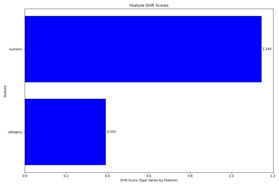
# Plot summary of drift across features
fig = plotter.plot_multiple()
plt.tight_layout()
plt.show()

(Source code, png, hires.png, pdf)

Feature-Level Distribution Comparison#

You can also examine the distribution shifts for individual features:

import numpy as np
import pandas as pd
import matplotlib.pyplot as plt
from tab_right.drift.drift_calculator import DriftCalculator
from tab_right.plotting.drift_plotter import DriftPlotter

# Generate datasets with drift
np.random.seed(42)
df1 = pd.DataFrame({
    'numeric': np.random.normal(0, 1, 100),
    'category': np.random.choice(['A', 'B', 'C'], 100, p=[0.5, 0.3, 0.2])
})

df2 = pd.DataFrame({
    'numeric': np.random.normal(1, 1.2, 120),
    'category': np.random.choice(['A', 'B', 'C'], 120, p=[0.2, 0.3, 0.5])
})

# Create calculator and plotter
drift_calc = DriftCalculator(df1, df2)
plotter = DriftPlotter(drift_calc)

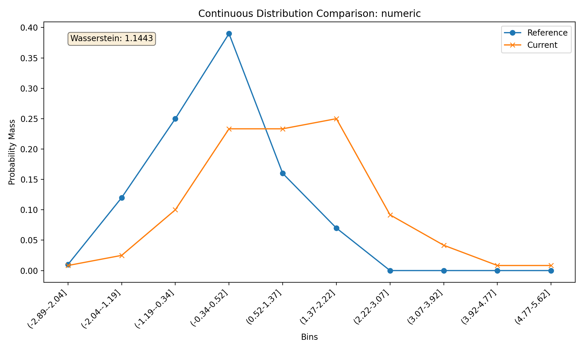
# Plot numerical feature distribution comparison
fig_numeric = plotter.plot_single('numeric')
plt.tight_layout()
plt.show()

(Source code, png, hires.png, pdf)

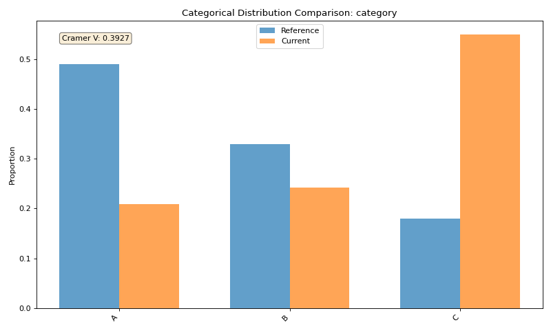
Categorical Feature Visualization#

Tab-right also makes it easy to visualize categorical feature drift:

import numpy as np
import pandas as pd
import matplotlib.pyplot as plt
from tab_right.drift.drift_calculator import DriftCalculator
from tab_right.plotting.drift_plotter import DriftPlotter

# Generate datasets with categorical drift
np.random.seed(42)
df1 = pd.DataFrame({
    'numeric': np.random.normal(0, 1, 100),
    'category': np.random.choice(['A', 'B', 'C'], 100, p=[0.5, 0.3, 0.2])
})

df2 = pd.DataFrame({
    'numeric': np.random.normal(1, 1.2, 120),
    'category': np.random.choice(['A', 'B', 'C'], 120, p=[0.2, 0.3, 0.5])
})

# Create calculator and plotter
drift_calc = DriftCalculator(df1, df2)
plotter = DriftPlotter(drift_calc)

# Plot categorical feature distribution comparison
fig_cat = plotter.plot_single('category')
plt.tight_layout()
plt.show()

(Source code, png, hires.png, pdf)

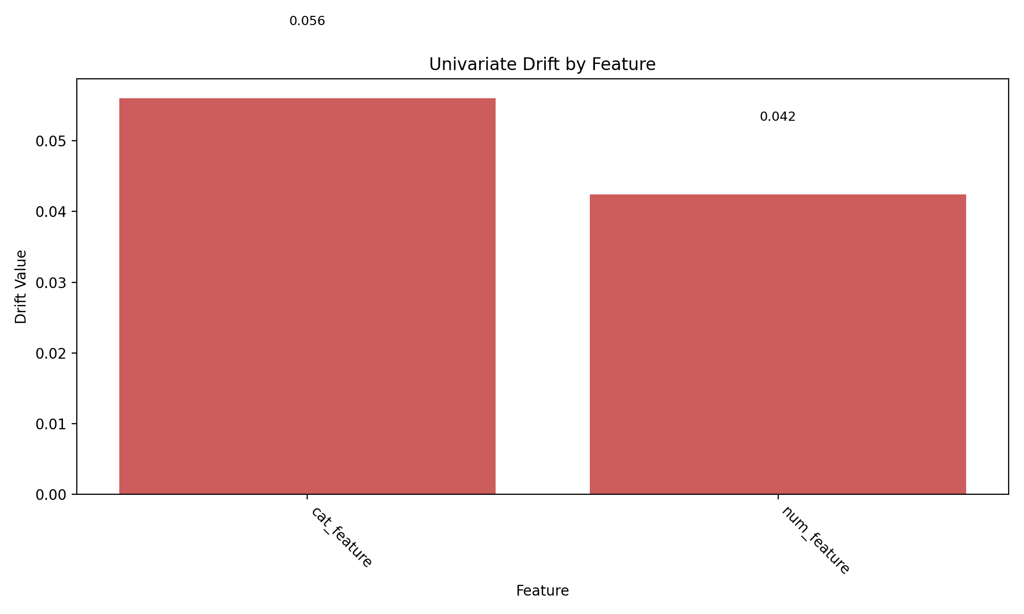
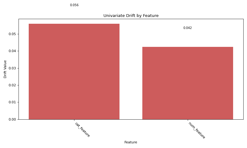
Direct Functions API#

For simpler use cases, tab-right also provides direct functions for drift analysis:

import numpy as np
import pandas as pd
import matplotlib.pyplot as plt
from tab_right.drift import univariate
from tab_right.plotting import DriftPlotter

# Generate datasets
np.random.seed(42)
df_ref = pd.DataFrame({
    'num_feature': np.random.normal(0, 1, 500),
    'cat_feature': np.random.choice(['A', 'B', 'C'], 500)
})

df_cur = pd.DataFrame({
    'num_feature': np.random.normal(0.3, 1.2, 500),
    'cat_feature': np.random.choice(['A', 'B', 'C'], 500, p=[0.2, 0.5, 0.3])
})

# Calculate drift across all features
result = univariate.detect_univariate_drift_df(df_ref, df_cur)

# Plot the results using DriftPlotter
fig = DriftPlotter.plot_drift_mp(None, result)
plt.tight_layout()
plt.show()

(Source code, png, hires.png, pdf)

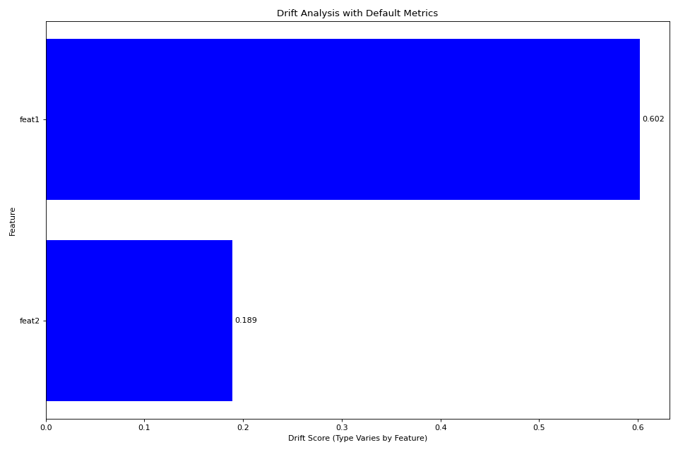
Working with Multiple Drift Metrics#

Tab-right supports various drift metrics that can be customized:

import pandas as pd
import numpy as np
import matplotlib.pyplot as plt
from tab_right.drift import univariate
from tab_right.drift.drift_calculator import DriftCalculator
from tab_right.plotting.drift_plotter import DriftPlotter

# Generate data
np.random.seed(42)
df_ref = pd.DataFrame({
    'feat1': np.random.normal(0, 1, 500),
    'feat2': np.random.choice(['A', 'B', 'C'], 500),
})

df_cur = pd.DataFrame({
    'feat1': np.random.normal(0.5, 1.5, 500),
    'feat2': np.random.choice(['A', 'B', 'C'], 500, p=[0.5, 0.3, 0.2]),
})

# Using DriftCalculator with default metrics
calc = DriftCalculator(df_ref, df_cur)

# Create a plotter
plotter = DriftPlotter(calc)

# Plot the results
fig = plotter.plot_multiple()
plt.title('Drift Analysis with Default Metrics')
plt.tight_layout()
plt.show()

(Source code, png, hires.png, pdf)

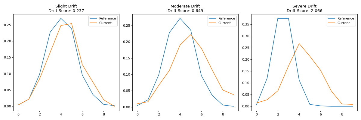
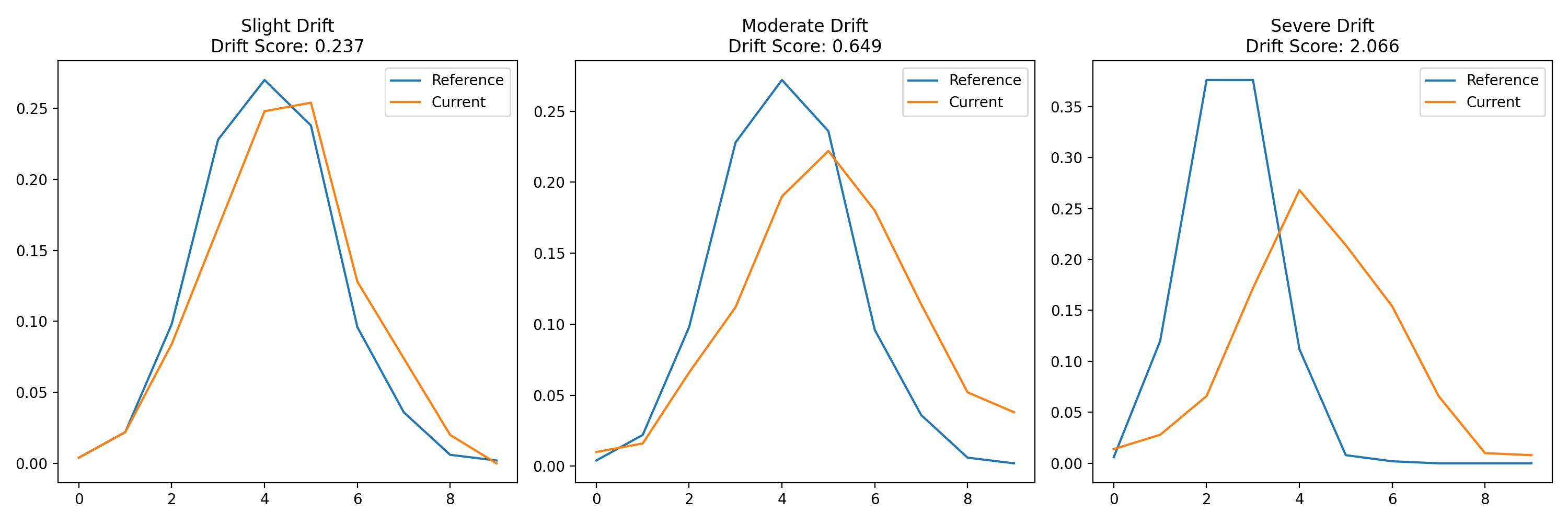
Visualizing Different Types of Drift#

Let’s look at how different degrees of drift appear in tab-right visualizations:

import pandas as pd
import numpy as np
import matplotlib.pyplot as plt
from tab_right.drift.drift_calculator import DriftCalculator
from tab_right.plotting.drift_plotter import DriftPlotter

# Create datasets with increasing levels of drift
np.random.seed(42)
ref_data = np.random.normal(0, 1, 500)

# Create three datasets with different levels of drift
slight_drift = np.random.normal(0.2, 1.1, 500)  # slight drift
moderate_drift = np.random.normal(0.5, 1.3, 500)  # moderate drift
severe_drift = np.random.normal(2.0, 1.8, 500)  # severe drift

# Create a figure with 3 subplots
fig, axes = plt.subplots(1, 3, figsize=(15, 5))

# Set up titles
titles = ['Slight Drift', 'Moderate Drift', 'Severe Drift']
drift_data = [slight_drift, moderate_drift, severe_drift]

# Create and plot each dataset using tab_right
for i, current_data in enumerate(drift_data):
    # Create DataFrames
    df_ref = pd.DataFrame({'value': ref_data})
    df_cur = pd.DataFrame({'value': current_data})

    # Calculate drift
    drift_calc = DriftCalculator(df_ref, df_cur)
    drift_result = drift_calc()
    drift_score = round(drift_result.iloc[0]['score'], 3)

    # Create plotter
    plotter = DriftPlotter(drift_calc)

    # Plot distribution on the corresponding subplot
    dist_fig = plotter.plot_single('value')

    # Remove the original figure and copy its content to our subplot
    for line in dist_fig.axes[0].lines:
        axes[i].plot(line.get_xdata(), line.get_ydata(),
                     color=line.get_color(), label=line.get_label())

    # Set title with drift score
    axes[i].set_title(f"{titles[i]}\nDrift Score: {drift_score}")
    axes[i].legend()

    # Close the original figure to prevent display
    plt.close(dist_fig)

plt.tight_layout()
plt.show()

(Source code, png, hires.png, pdf)

Key Features of tab-right’s Drift Detection#

Tab-right offers comprehensive drift detection capabilities:

Flexible API: Choose between object-oriented (DriftCalculator/DriftPlotter) or functional approaches
Automatic feature type detection: Appropriate metrics are selected based on the data type
Multiple drift metrics: Including Wasserstein distance, KS test, and Cramer’s V
Matplotlib integration: Create publication-ready plots with built-in matplotlib figures
Multi-feature analysis: Analyze drift across all features at once
Probability density comparison: Examine detailed distribution changes

These tools make it easy to track and analyze distribution shifts in your data, helping you maintain model performance over time.

Drift Detection#

Drift Detection with tab-right#

Available Drift Metrics#

Example: Using DriftCalculator and DriftPlotter#

Feature-Level Distribution Comparison#

Categorical Feature Visualization#

Direct Functions API#

Working with Multiple Drift Metrics#

Visualizing Different Types of Drift#

Key Features of tab-right’s Drift Detection#

This Page